Box Plot vs Histogram: Same Quartiles, Different Shapes
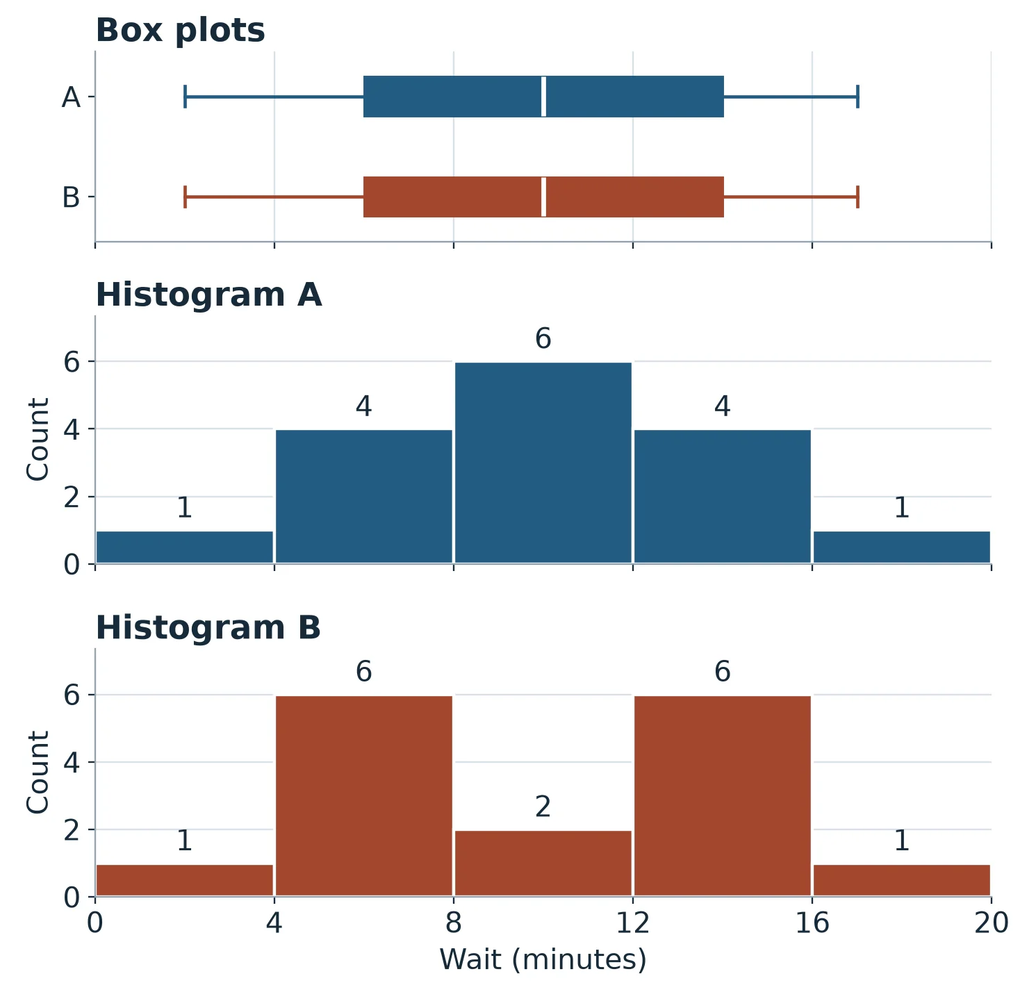
At checkout A, six customers waited at least 8 minutes and less than 12. At checkout B, only two did. Both sets of 16 example waits have a median of 10 minutes and produce identical box plots.
Use a box plot to compare medians and the spread of the middle half of each group. Use a histogram to see peaks, gaps, and how many observations fall in each interval.
What the identical box plots show
Each row lists 16 invented checkout waits in minutes, from shortest to longest.
| Checkout | Wait times (minutes) |
|---|---|
| A | 2, 4, 5, 6, 6, 9, 9, 10, 10, 10, 11, 14, 14, 15, 15, 17 |
| B | 2, 6, 6, 6, 6, 6, 6, 10, 10, 14, 14, 14, 14, 14, 14, 17 |
For each checkout, average the 8th and 9th waits to get the median. Take the median of the lower eight waits for the first quartile (Q1) and the median of the upper eight for the third quartile (Q3).
Both groups have the same five-number summary in minutes, with a minimum of 2, Q1 of 6, a median of 10, Q3 of 14, and a maximum of 17. The boxes run from 6 to 14 with a median line at 10. The distance between Q1 and Q3 is the interquartile range (IQR), here 14 − 6 = 8 minutes.
A simple box plot extends its whiskers to the minimum and maximum. A modified box plot uses two cutoffs called fences. Subtract 1.5 × IQR from Q1 for the lower fence (6 − 12 = −6 minutes) and add that amount to Q3 for the upper fence (14 + 12 = 26 minutes).
The modified whiskers reach the smallest and largest observed waits at or between the fences. Here those waits are 2 and 17 minutes for both groups. Points beyond either fence appear separately as potential outliers. Penn State’s guide to standard and modified box plots
What the histograms show with four-minute bins
Both histograms start at 0 and use the same four-minute bins and axis scales so you can compare bar heights directly. Each bin includes its starting value and excludes its ending value. For example, [8, 12) counts waits of at least 8 minutes and less than 12. The bar height is the number of waits in that interval. NIST’s guide to histograms
| Wait (minutes) | A count | B count |
|---|---|---|
| [0, 4) | 1 | 1 |
| [4, 8) | 4 | 6 |
| [8, 12) | 6 | 2 |
| [12, 16) | 4 | 6 |
| [16, 20) | 1 | 1 |
A’s tallest bar spans 8 to under 12 minutes. B’s two tallest bars span 4 to under 8 and 12 to under 16, with six waits in each and a dip to two waits in between. The box plots summarize both patterns with the same five values.
Try a wider bin and a longer wait
- Which four-minute bin contains A’s wait of exactly 4 minutes? How many of A’s waits are in that bin?
- Count B’s waits in three eight-minute bins starting at 0. Use [0, 8), [8, 16), and [16, 24). Does the wider histogram still show the dip?
- Replace A’s 17-minute wait with a 31-minute wait. Using Q1 = 6 and Q3 = 14, where does the upper whisker of a modified box plot end? How would you mark the 31-minute wait?
Worked answers
- The 4-minute wait goes in [4, 8). A has four waits there, at 4, 5, 6, and 6 minutes.
- The counts are 7, 8, and 1, from 1 + 6, 2 + 6, and the single 17-minute wait. The middle eight-minute bin combines the dip with the peak to its right, so the dip disappears. The two peaks describe the four-minute histogram of these example waits.
- The upper fence is 26 minutes. The upper whisker ends at 15 minutes, the largest observed wait within the fences. Mark 31 minutes separately as a potential outlier. A simple box plot would extend its upper whisker to 31 minutes.
Practice the whisker rule from memory
If you put the whisker at 26, try this flashcard. “The upper fence is 26 minutes and the two longest waits are 15 and 31 minutes. Where does the upper whisker of a modified box plot end?” Say the endpoint and give the reason before checking your answer. Try recalling it tomorrow and again a few days later. Spacing out those attempts can help you remember the rule. Karpicke and Bauernschmidt’s experiment on spaced retrieval
The English AP Statistics deck has prompts on where whiskers end and how to calculate fences. AP Statistics flashcards
AP Statistics covers how to compare distributions with these displays in Unit 1, Topic 1.9. College Board’s course framework · AP Statistics study plan
Prepared with AI assistance using invented wait times. The quartiles, whiskers, and bin counts were checked with Python.